Practical N°2

3D projection alignment and CTF correction on simulated micrographs of Lumbricus terrestris giant hemoglobin

Introduction

For this practical session, we will need some files kept in "TP2.zip" (click with left button of your mouse to download it or send me an email if you have trouble getting it), and we will need to define a working directory and several subdirectories:
1- Creation of the working directory : type "unzip TP2.zip". This should create the subdirectoryTP2 with subdirectory makedata which contains the batch b01.mkd. plus six subdirectories named: micrographs, batch, doc, images, r2d, and r3d. if you don't have the file TP2.zip, ask me to send it to you by email (size: 3.5 Mo).
4- For traveling from subdirectory to an other, you can type the following orders:
    to see where you are type : "pwd"
    to go from TP2 to TP2/micrographs type : "cd micrographs"
    to go from  TP2/micrographs to TP2/images, type : "cd ../images"
    to go from TP2/images to TP2, type : "cd .."
5- In this tutorial, we will use two softwares "spider" and "web". The spider version used here is the latest released by Joachim Frank "VERSION:  UNIX  14.16    ISSUED: 03/30/2006". For information about this latest version of spider and web contact the Wadsworth Center for Laboratories and Research (Pr J. Franck), and visit their web site http://www.wadsworth.org/spider_doc/spider/docs/master.html .

1. Simulating four cryo-EM images of lumbricus

The batch b01.mkd was designed to simulate four micrographs containing each 120 hemoglobin 2D projections with an even angular distribution (every 5°). The experimental conditions to create those images are resumed in the following table :

Pixel size in A	3,5 A
Cs of the objective lens	0.5 mm
defocus value in A	in the ranges of -25000 to -40000 Angstroems underfocused
Lambda value	0.02508 for an acceleration voltage of 200 kV
Maximum spatial frequency	(1/2*Pixel size in A) = (1/2*3.5)= 0.142857 A-1
Source size in A-1	0.00431 A-1
defocus spread	100 A
Astigmatism value	0.0 A
Astigmatism azimuth	0°
amplitude contrast ratio	0.07
enveloppe halfwidth in A-1	0.07
undefocused	-1

The batch b01.mkd produces four micrographs ../Micrographs/MIC[001-004].hbl and their reduced copy termed ../Micrographs/PIC[001-004].hbl.

PIC001.hbl	PIC002.hbl	PIC003.hbl	PIC004.hbl

These simulated micrographs were obtained by multiplying in reciprocal space each fantom image of a micrograph, with a specidific contrast transfert function.

	tfd001.hbl	tfd002.hbl	tfd003.hbl	tfd004.hbl

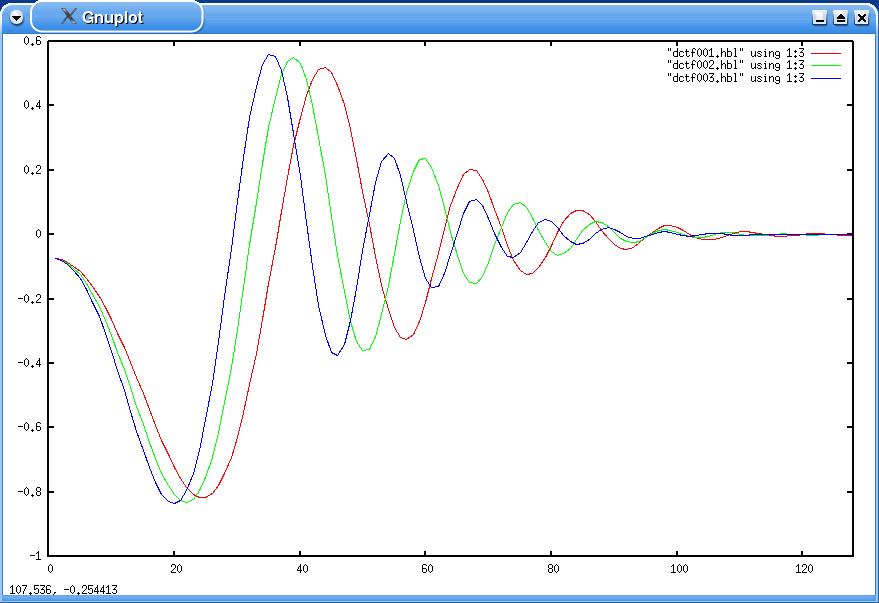
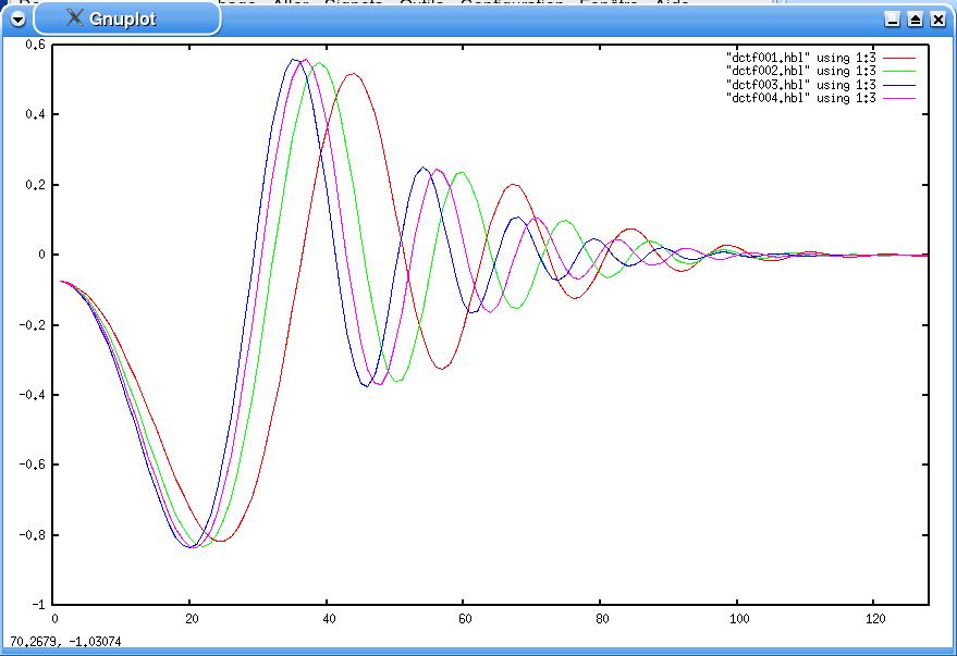
While looking at the radial profiles of the three first CTFs what troubles can you imagine and for which spacial frequencies ?

gnuplot
set xrange [0:128
set yrange [-1.:0.6]
plot "dctf001.hbl" using 1:3 with line, "dctf002.hbl" using 1:3 with line, "dctf003.hbl" using 1:3 with line

 

Will the fourth data set improve the situation?

gnuplot
set xrange[0:128
set yrange [-1.:0.6]
plot "dctf001.hbl" using 1:3 with line, "dctf002.hbl" using 1:3 with line, "dctf003.hbl" using 1:3 with line, "dctf004.hbl" using 1:3 with line

 

1. Interactive particle picking

You need first to pick the particles from each micrograph. You can do this interactively using Web (or other avaible display programs). You can also see why automatic partic picking becomes a pressing issue now in the field of single particles.

Using the Web software, you can use the operation "display image" to get one of the reduced micrographs [PIC001-004.hbl] on the screen. Then, you can use the operation "Pixel" using the following operations:

Activate : Save Selections in doc. file

Doc file : ../doc/dmic001

Activate option "inside last image"

Activate option "leave marker"

Key N°: 1

X Reg: 1 YReg : 2

Radius = 21

Accept

 

You can select all the particles by clicking on their center with the left button of the mouse. To stop the operation you can click on the right button. A white circle will appear on selected particles to avoir picking twice the same particle.   Watch out ! The web software might still have this bug ! For soe operations, Web will create files who by default will have the extension ".DAT" rather then the one you types (e.g., ".hbl").

2. windowing of the images in 4 sets of images

Then, the batch b17.fed will be used to perform the windowing of the 4x120 images from the four micrographs (MIC[001-004].hbl).

If the batch functions correctely, you should end up with a series of 120 100x100 pixels images per micrograph.

3. Estimation of the defocus of each micrograph from its averaged power spectrum

You will need to run 4 times the batch b18.fed to compute the averaged power spectra of the four micrographs (../r2d/POW[001-004].hbl) and to compute the doc files of their radially averaged densities (../doc/dpws[001-004].hbl). Each time you will need to change the value of the register x99 (from 1 to 4).

../r2d/Pow001.hbl	../r2d/Pow002.hbl	../r2d/Pow003.hbl	../r2d/Pow004.hbl

Remark: At this steage please start the batch b19.fed (which prepares a 3D mask and a reference volume) and above all, b20.fed who computes three cycles of aligment on our four sets of images. Indeed, this alignment takes some time (30 minutes on my machine) and the computations may be running while we will continue in interactive mode the exploration of the CTF and of the power spectra.

Interactive dtermination of the defocus of each micrograph

At this stage, we use the Web software and start the operation "CTF from doc. file". You have then to select one of the four radialy averaged profile of the power spectra computed by b18.fed (../doc/dpws[001-004].hbl). A small window appears and asks for additional values:

Pixel size : in our case 3.5 A
Spherical abberation : in our case 0.5 mm	Electron Energy kev : in our case 200kV
Source size : in our case 0.00431 A-1	Defocus spread : in our case 100 A
Amplitude contrast : 0.07 (7% for cryoEM, ~12% for negative staining)
Gaussian envelope Halfwidth : in our case 0.07

When thee values are accepted, the experimental profile comming from the power spectrum doc file appears above a theoretical profile CTF curve. On this screen, a set of vertical lines apprear each time the CTF curve crosses the zero line (along X horizontal axisof the image). By adjusting the defocus value, we have to make sure these vertical lines correspond to the local minima of the power spectrum radial average.

For this, a small window is open by the program Web which contains three cursors :

Def 0-70,000 (A)	cursor
Def 0-1000 (A)	cursor
Plot cutoff percentage	cursor

By adjusting the position of the cursors, we can obtain a good superposition of the zeros of CTF with the local minima of the power spectrum (See below).

Remark: You should also use the operation TF ED developped by Pawel Penczek wich estimates the defocus but also the astigmatism parameters. This operation is very accurate and put into a do loop, it can be used to get automatically and without manual fitting the defocus of each micrograph.

The batch b23.fed will help you to produce theoretical profiles in document files (dapws[001-004].hbl), corresponding to the defocuses you will have found for the power spectra of your micrographs.

Results of the alignment

When the batch b20.fed is finished, we can check the resolution doc files for a given set of images (here micrograph 4) and for the three cycles of alignment

../doc/dresol101.hbl, ../doc/dresol102.hbl, ../doc/dresol103.hbl	at cycle N°3 Resolution limit of 0.5 = 21,10A (Fq=0,16580)
../doc/dresol201.hbl, ../doc/dresol202.hbl, ../doc/dresol203.hbl	at cycle N°3 Resolution limit of 0.5 = 20,93A (Fq=0,16717)
../doc/dresol301.hbl, ../doc/dresol302.hbl, ../doc/dresol303.hbl	at cycle N°3 Resolution limit of 0.5 = 19,08A (Fq=0,18333)
../doc/dresol401.hbl, ../doc/dresol402.hbl, ../doc/dresol403.hbl	at cycle N°3 Resolution limit of 0.5 = 19,02A (Fq=0,18390)

In this exemple; the volume seem to have improved from cycle 1 to cycle 3. A good way to display the resolution curves, is to use the gnuplot sofware. Example: to see the resolution curves for the 3 alignment cycle on a given group, try the following orders

gnuplot
set xrange [0:0.5]
plot "../doc/dresol101.hbl" using 3:5 with line , "../doc/dresol102.hbl" using 3:5 with line , "../doc/dresol103.hbl" using 3:5 with line 
plot "../doc/dresol201.hbl" using 3:5 with line , "../doc/dresol202.hbl" using 3:5 with line , "../doc/dresol203.hbl" using 3:5 with line 
plot "../doc/dresol301.hbl" using 3:5 with line , "../doc/dresol302.hbl" using 3:5 with line , "../doc/dresol303.hbl" using 3:5 with line 
plot "../doc/dresol401.hbl" using 3:5 with line , "../doc/dresol402.hbl" using 3:5 with line , "../doc/dresol403.hbl" using 3:5 with line 

The resolution curves show for Fourier units from 0 to 0.5 (see Fourrier units conventions in TP1), a correlation value found between two volumes computed from odd and even sub-populations of 2D images. This value usually starts around 1.0 and slowly degrade and oscillate around 0.0 for high spatial frequencies. However, we can see here a series of local minima in the curve. According to you what is the reason for these local minima ?

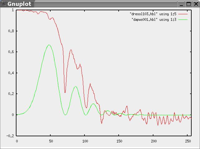
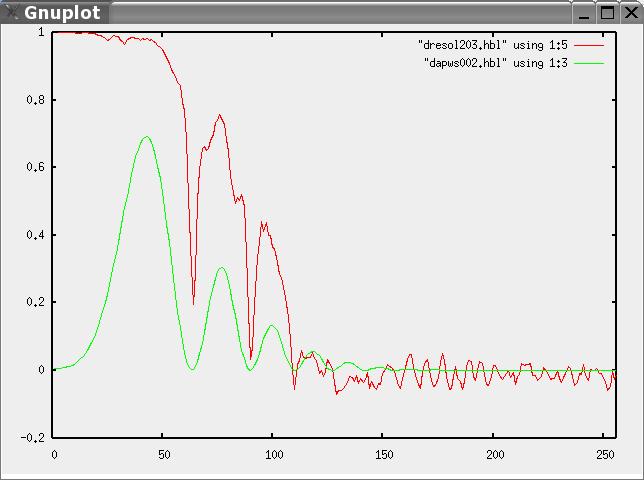
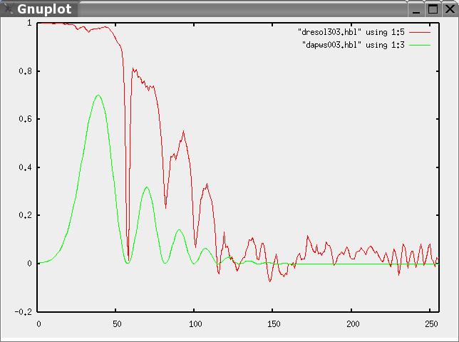
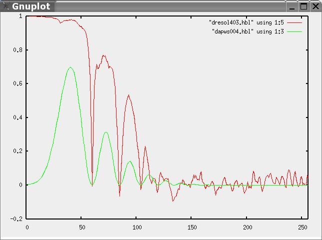
The following gnuplot orders will help you to display the same resolution doc files with the profiles of the theoretical power spectra that you calculated with b23.fed after measuring the defocus of each micrograph. Local minima coincide in both curves. What does it mean ?

 

gnuplot

set xrange [0:256]
set yrange [-0.2:1.0]
plot "../doc/dresol103.hbl" using 1:5 with line , "../doc/dapws001.hbl" using 1:3 with line , "../doc/dresol103.hbl" using 1:6 with line 
plot "../doc/dresol203.hbl" using 1:5 with line , "../doc/dapws002.hbl" using 1:3 with line , "../doc/dresol203.hbl" using 1:6 with line 
plot "../doc/dresol303.hbl" using 1:5 with line , "../doc/dapws003.hbl" using 1:3 with line , "../doc/dresol303.hbl" using 1:6 with line 
plot "../doc/dresol403.hbl" using 1:5 with line , "../doc/dapws004.hbl" using 1:3 with line , "../doc/dresol403.hbl" using 1:6 with line 

Or use surface rendering with Web or using Chimera.

When the alignment of the image sets is performed by the batch b20.fed , we can compute the Wiener filtering on the aligne images (from cycle 3). This is done by the batch b21.fed . In comparison, the batch b22.fed provides the ideal solution (if centering of the images and determination of their eulerian angles were perfectly correct).

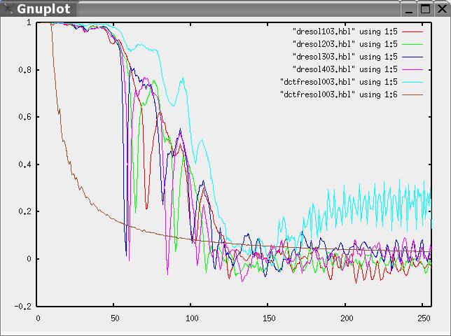
One can see on the resolution doc file after CTF correction has a much better resolution. Small local minima can be found in the curve "dctfresol003.hbl". How do you explain such local minima ? How would you do to remove them ?

 

gnuplot
set xrange [0:256]
set yrange [-0.2:1.0]

plot "../doc/dresol103.hbl" using 1:5 with line , "../doc/dresol203.hbl" using 1:5 with line , "../doc/dresol303.hbl" using 1:5 with line , \
"../doc/dresol403.hbl" using 1:5 with line , "dctfresol003.hbl" using 1:5 with lin, "dctfresol003.hbl" using 1:6 with lin

Here again Chimera and Web can be used to compared the CTF corrected volume with the non corrected ones.

Volume names	Defocus Group and Alignment cycle N°	batches
../r3d/vol103.hbl	groupe # 1 and alignment cycle # 3	(b20.fed )
../r3d/vol203.hbl	groupe # 2 and alignment cycle # 3	(b20.fed )
../r3d/vol303.hbl	groupe # 3 and alignment cycle # 3	(b20.fed )
../r3d/vol403.hbl	groupe # 4 and alignment cycle # 3	(b20.fed )
../r3d/vctf003.hbl	global CTF corrected volume groups #1-4 and alignment cycle #3	(b21.fed )
../r3d/vhpctf003.hbl	same as previous line after high-pass filtered (Rf=0.08, T°C=0.02)	(b22.fed )

Using Chimera you can also compare the volumes, but as the differences are small and very local you might not see as well as in the slices extracted from the volumes.

 

At this stage you can compare your resolution curve from CTF corrected volumes at cycle N°3 with the resolution curve computed from the ideally aligned images (b22.fed ). If you see a difference, propose solutions to improve the quality of the alignment and CTF correction:

Propositions:

For more elaborate 3D reconstruction schemes check the spider web site and more specifically the techniques section on projection matching or on CTF correction. and contact the spider group which will help you for solving specific problems.

Finally, we hope this rapid tutorial helped you in your first CTF corrected 3D reconstruction of a single particle, and we wish you good luck for your own research projects !

Friendly yours,
Nicolas

(Please send us your comments by email at "Nicolas.Boisset@impmc.jussieu.fr"and "Ricardo.Aramayo@impmc.jussieu.fr"to help us improve this tutorial).